
Image resampling methods
When a geospatial image is displayed at a zoom level or resolution that differs from its source, the rendering engine must compute new pixel values from the original data. This process is called resampling. The method you choose determines whether the output prioritises value fidelity, visual smoothness, or edge sharpness.
What is resampling?
Geospatial images are stored as rasters — grids of pixels, each holding a value at a fixed spatial resolution. When the image is rendered at a different resolution (zoomed in, zoomed out, or reprojected to a different coordinate system), the source pixel grid no longer aligns perfectly with the output pixel grid.
Resampling is the algorithm that bridges this gap: for each output pixel, it looks at nearby source pixels and decides what value to assign. Different algorithms make different trade-offs between accuracy, smoothness, and computational cost.
The four methods
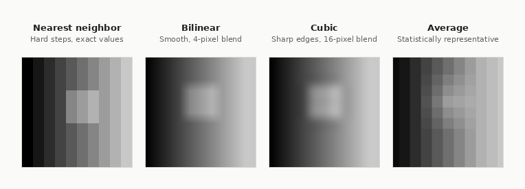
Nearest neighbor
For each output pixel, the algorithm finds the single closest source pixel and copies its value directly. No calculation is performed — the output value is always an exact copy of a source value.
- Reads 1 source pixel per output pixel — fastest of the four methods
- Output values are always present in the original dataset — no new values are introduced
- Produces a stepped, blocky appearance on continuous imagery when upsampling significantly
When to use: The only method suitable for rasters where pixel values are labels — segmentation masks, annotation layers, land-use maps. Because it never blends values, class boundaries are preserved exactly and output values always map to a valid label.
Bilinear
The output pixel value is computed as a distance-weighted average of the 4 nearest source pixels. Pixels closer to the output pixel centre contribute more to the result.
- Reads 4 source pixels per output pixel
- Produces smooth, continuous transitions — well-suited to data that varies gradually across space
- Output values are interpolated and may not match any value in the source dataset
When to use: Best for rasters where pixel values are measurements — elevation, temperature, reflectance, orthophoto RGB. Any data where interpolating between two values produces a meaningful result.
Cubic
The output pixel is computed from the 16 nearest source pixels using a bicubic polynomial. The wider sampling window allows the algorithm to model curvature in the data, producing sharper edges than bilinear.
- Reads 16 source pixels per output pixel — most compute-intensive
- Preserves and enhances fine detail and edge sharpness better than bilinear
- Can produce slight ringing artefacts (overshoot) near high-contrast edges
- Output values are interpolated and may not match any value in the source dataset
When to use: Best for high-resolution optical imagery — aerial orthophotos, high-res satellite bands — where preserving fine spatial detail matters more than computation cost.
Average
The output pixel value is the arithmetic mean of all source pixels that fall within the corresponding source area. As the zoom level decreases (more source pixels map to a single output pixel), more values are averaged together.
- Number of source pixels read scales with the downsampling ratio
- Prevents aliasing artefacts that nearest neighbor produces at small scales
- Maintains the statistical properties of the data across zoom levels
When to use: Recommended when downsampling significantly — zooming far out, building image overviews, or generating pyramid levels. It produces the most statistically representative result for measurement data at small scales.
Choosing the right method
| Method | Pixel values are | Typical use cases | Visual result | Cost |
|---|---|---|---|---|
| Nearest neighbor | Labels or measurements | Segmentation masks, annotation layers, land-use maps | Blocky / stepped | Lowest — 1 px read |
| Bilinear | Measurements only | Elevation models, temperature grids, multispectral bands, orthophotos | Smooth | Low — 4 px read |
| Cubic | Measurements only | Aerial orthophotos, high-res optical imagery | Sharp, detailed | Higher — 16 px read |
| Average | Measurements only | Zoomed-out overviews, downsampling, image pyramids | Blended, no aliasing | Scales with zoom |
Only nearest neighbor is safe when pixel values are labels. Bilinear, cubic, and average all compute new values by blending neighbours. If your raster encodes categories — where
1means "building" and3means "vegetation" — blending could produce2.0, which maps to "road" even if there is no road. The algorithm has no way to know the values are identifiers, not measurements. Use nearest neighbor any time pixel values represent labels rather than quantities.
Updated 2 months ago